Table of Contents
Confidence Intervals for $R^2$ in Meta-Regression Models
The $R^2$ statistic that is shown in the output for meta-regression models (fitted with the rma() function) estimates how much of the total amount of heterogeneity is accounted for by the moderator(s) included in the model (Raudenbush, 2009). An explanation of how this statistic is computed is provided here.
Based on a simulation study, we know that the $R^2$ statistic is not very accurate unless the number of studies ($k$) is quite large (López-López et al., 2014). To gauge the precision of the value of $R^2$ in a particular meta-analysis, we may want to compute a confidence interval (CI) for this statistic. However, this is difficult, because the $R^2$ statistic is based on the ratio of two heterogeneity estimates, one from the random-effects model (to obtain an estimate of the total amount of heterogeneity) and the other from the mixed-effects meta-regression model (to obtain an estimate of the residual amount of heterogeneity) that need to be fitted in turn. A possible approach we can take to construct a CI for $R^2$ is to use bootstrapping. This is illustrated below (see also here for an illustration of using bootstrapping in the context of the random-effects model).
Data Preparation / Inspection
For this example, we will use the data from the meta-analysis by Bangert-Drowns et al. (2004) on the effectiveness of writing-to-learn interventions on academic achievement. For the purposes of this example, we will keep only the columns needed and only the rows where the moderators to be used in the meta-regression model below are completely coded (this results in two rows being removed from the dataset; note that these two rows would be removed anyway when fitting the model, but for bootstrapping, it is better to remove these rows manually beforehand).
dat <- dat.bangertdrowns2004
dat <- dat[c(1:3,9:12,15:16)]
dat <- dat[complete.cases(dat),]
head(dat)
  id   author year info pers imag meta     yi    vi
1  1 Ashworth 1992    1    1    0    1  0.650 0.070
2  2    Ayers 1993    1    1    1    0 -0.750 0.126
3  3   Baisch 1990    1    1    0    1 -0.210 0.042
4  4    Baker 1994    1    0    0    0 -0.040 0.019
5  5   Bauman 1992    1    1    0    1  0.230 0.022
6  6   Becker 1996    0    1    0    0  0.030 0.009
7  .        .    .    .    .    .    .      .     .
Variable yi provides the standardized mean differences and vi the corresponding sampling variances. Variables info, pers, imag, and meta are dummy variables to indicate whether the writing-to-learn intervention contained informational components, personal components, imaginative components, and prompts for metacognitive reflection, respectively (for the specific meaning of these variables, see Bangert-Drowns et al., 2004). We will use these 4 dummy variables as potential moderators.
Meta-Regression Model
We start by fitting the meta-regression model containing these 4 moderators as follows:
res <- rma(yi, vi, mods = ~ info + pers + imag + meta, data=dat)
res
Mixed-Effects Model (k = 46; tau^2 estimator: REML)

tau^2 (estimated amount of residual heterogeneity):     0.0412 (SE = 0.0192)
tau (square root of estimated tau^2 value):             0.2030
I^2 (residual heterogeneity / unaccounted variability): 51.71%
H^2 (unaccounted variability / sampling variability):   2.07
R^2 (amount of heterogeneity accounted for):            18.34%

Test for Residual Heterogeneity:
QE(df = 41) = 82.7977, p-val = 0.0001

Test of Moderators (coefficients 2:5):
QM(df = 4) = 10.0061, p-val = 0.0403

Model Results:

         estimate      se     zval    pval    ci.lb   ci.ub
intrcpt    0.3440  0.2179   1.5784  0.1145  -0.0831  0.7711
info      -0.1988  0.2106  -0.9438  0.3453  -0.6115  0.2140
pers      -0.3223  0.1782  -1.8094  0.0704  -0.6715  0.0268   .
imag       0.2540  0.2023   1.2557  0.2092  -0.1424  0.6504
meta       0.4817  0.1678   2.8708  0.0041   0.1528  0.8106  **

---
Signif. codes:  0 '***' 0.001 '**' 0.01 '*' 0.05 '.' 0.1 ' ' 1
The omnibus test indicates that we can reject the null hypothesis that the 4 coefficients corresponding to these moderators are all simultaneously equal to zero ($Q_M(\textrm{df} = 4) = 10.01, p = .04$). Moreover, it appears that writing-to-learn interventions tend to be more effective on average when they include prompts for metacognitive reflection ($p = .0041$, with a coefficient that indicates that the size of the effect is on average 0.48 points higher when such prompts are given). Finally, the results indicate that around $R^2 = 18.3\%$ of the heterogeneity is accounted for by this model.
Bootstrap Confidence Interval
We will now use (non-parametric) bootstrapping to obtain a CI for $R^2$. For this, we load the boot package and write a short function with three inputs: the first provides the original data, the second is a vector of indices which defines the bootstrap sample, and the third is the formula for the model to be fitted. The function then fits the same meta-regression model as above based on the bootstrap sample and returns the value of the $R^2$ statistic. The purpose of the try() function is to catch cases where the model fitting algorithm does not converge.
library(boot)

boot.func <- function(dat, indices, formula) {
   res <- try(suppressWarnings(rma(yi, vi, mods = formula, data=dat[indices,])), silent=TRUE)
   if (inherits(res, "try-error")) NA else res$R2
}
The actual bootstrapping (based on 10,000 bootstrap samples) can then be carried out with:1)
set.seed(1234)
res.boot <- boot(dat, boot.func, R=10000, formula=formula(res))
Now we can obtain various types of CIs (by default, 95% CIs are provided):
boot.ci(res.boot, type=c("norm", "basic", "perc", "bca"))
BOOTSTRAP CONFIDENCE INTERVAL CALCULATIONS
Based on 9998 bootstrap replicates

CALL :
boot.ci(boot.out = res.boot, type = c("norm", "basic", "perc", "bca"))

Intervals :
Level      Normal              Basic
95%   (-54.04,  52.07 )   (-63.30,  36.69 )

Level     Percentile            BCa
95%   ( 0.00, 99.99 )   ( 0.00, 57.59 )
Calculations and Intervals on Original Scale
We see that the results are based on 9,998 bootstrap replicates, so apparently for two of the bootstrap samples the model fitting algorithm did not converge. Since this happened so infrequently, we can ignore this issue.
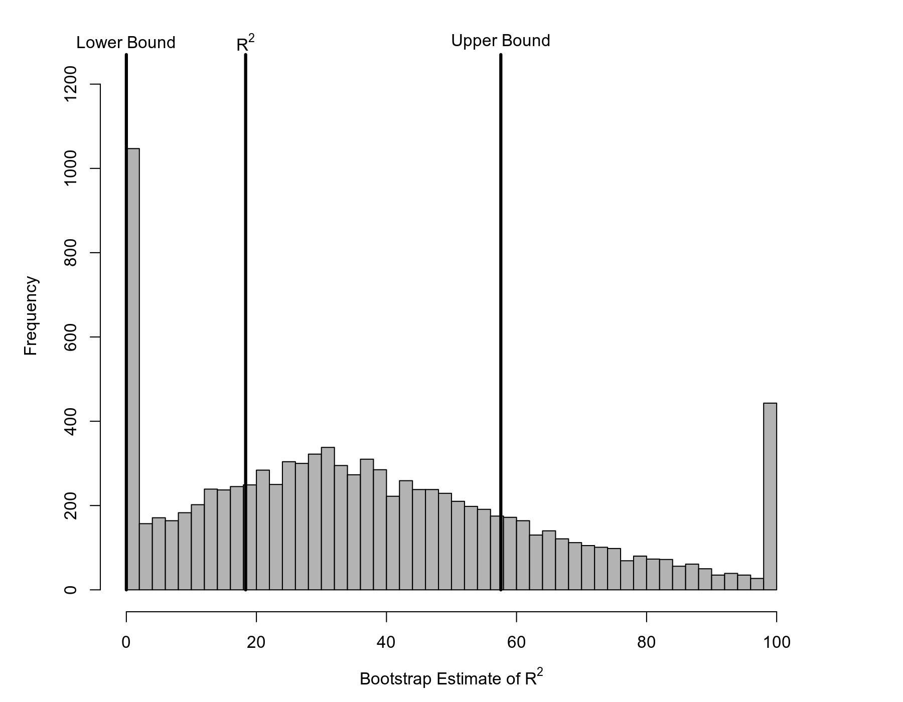
Furthermore, note that some of the CIs yield a negative lower bound. While we could simply treat these lower bounds as zero (since the value of the $R^2$ statistic must fall between 0 and 100), we can avoid this issue by focusing on the percentile or the so-called bias-corrected and accelerated (BCa) CIs. There are typically good reasons for preferring the latter, which yields the bounds $0\%$ to $57.6\%$. This is a rather wide interval, indicating that even with $k = 46$ studies, the $R^2$ statistic obtained is not very accurate.
The figure below shows that the bootstrap distribution has a peculiar shape, with peaks at $0\%$ and $100\%$ and a slightly right-skewed distribution in-between.
Conclusions
As the example above demonstrates, the value of $R^2$ obtained from a meta-regression model can be quite inaccurate and hence should be treated with due caution. At the same time, it should be noted that the accuracy of using bootstrapping for constructing CIs for $R^2$ in meta-regression models has not been examined previously. Therefore, I conducted a simulation study to examine the coverage of the various CIs shown above for various values of $k$ and true $R^2$ (Viechtbauer, 2023; you can find the slides for this conference talk here). The results indicate that the coverage of the BCa method is actually quite acceptable, although it can be a bit conservative (i.e., too wide), especially when $k$ is small or the true $R^2$ value is close to zero.2)
Addendum
The same principle also works for more complex models (such as those that can be fitted with the rma.mv() function). The $R^2$ statistic, which is simply the proportional reduction in the variance component when adding the moderator(s) to the model, can also be computed when the model contains multiple variance components. An example to illustrate this for a multilevel model is provided here. The example also shows how to make use of parallel processing to speed up the bootstrapping.
References
Bangert-Drowns, R. L., Hurley, M. M. & Wilkinson, B. (2004). The effects of school-based writing-to-learn interventions on academic achievement: A meta-analysis. Review of Educational Research, 74(1), 29-58. https://doi.org/10.3102/00346543074001029
López-López, J. A., Marín-Martínez, F., Sánchez-Meca, J., Van den Noortgate, W. & Viechtbauer, W. (2014). Estimation of the predictive power of the model in mixed-effects meta-regression: A simulation study. British Journal of Mathematical and Statistical Psychology, 67(1), 30-48. https://doi.org/10.1111/bmsp.12002
Raudenbush, S. W. (2009). Analyzing effect sizes: Random effects models. In H. Cooper, L. V. Hedges, & J. C. Valentine (Eds.), The handbook of research synthesis and meta-analysis (2nd ed., pp. 295–315). New York: Russell Sage Foundation.
Viechtbauer, W. (2023). Confidence intervals for the amount of heterogeneity accounted for in meta-regression models. European Congress of Methodology, Ghent, Belgium.