Table of Contents
Difference Between the Omnibus Test and Tests of Individual Predictors
When a meta-regression model includes multiple predictors, one can examine the significance of each individual predictor (i.e., coefficient), but also the significance of the model as whole. For the latter, we can conduct an omnibus test that tests the null hypothesis that all predictors are unrelated to the effect sizes. It can happen that the omnibus test is not significant, yet some of the individual coefficients are. The reverse can also happen where the omnibus test is significant, but none of the individual predictors are. Let's consider some examples to illustrate these cases.
Non-Significant Omnibus Test but Significant Predictors
For this example, we will work with the data from the meta-analysis by Bangert-Drowns et al. (2004) on the effectiveness of school-based writing-to-learn interventions on academic achievement. In each of the studies included in this meta-analysis, an experimental group (i.e., a group of students that received instruction with increased emphasis on writing tasks) was compared against a control group (i.e., a group of students that received conventional instruction) with respect to some content-related measure of academic achievement (e.g., final grade, an exam/quiz/test score).
library(metafor)
dat <- dat.bangertdrowns2004
dat
 id      author year grade length .  ni    yi    vi
  1    Ashworth 1992     4     15 .  60  0.65 0.070
  2       Ayers 1993     2     10 .  34 -0.75 0.126
  3      Baisch 1990     2      2 .  95 -0.21 0.042
  4       Baker 1994     4      9 . 209 -0.04 0.019
  5      Bauman 1992     1     14 . 182  0.23 0.022
  6      Becker 1996     4      1 . 462  0.03 0.009
  7 Bell & Bell 1985     3      4 .  38  0.26 0.106
  8     Brodney 1994     1     15 . 542  0.06 0.007
  9      Burton 1986     4      4 .  99  0.06 0.040
 10   Davis, BH 1990     1      9 .  77  0.12 0.052
  .           .    .     .      . .   .     .     .
 45       Wells 1986     1      8 . 250  0.04 0.016
 46      Willey 1988     3     15 .  51  1.46 0.099
 47      Willey 1988     2     15 .  46  0.04 0.087
 48   Youngberg 1989     4     15 .  56  0.25 0.072
Variable yi provides the standardized mean differences (with positive values indicating a higher mean level of academic achievement in the intervention group), while variable vi provides the corresponding sampling variances.
We will now examine whether there is evidence that the effectiveness of writing-to-learn interventions differs across grade levels. The grade variable is coded numerically (1 = elementary, 2 = middle, 3 = high-school, 4 = college), but we will treat it as a factor variable.
res <- rma(yi, vi, mods = ~ factor(grade), data=dat)
res
Mixed-Effects Model (k = 48; tau^2 estimator: REML)

tau^2 (estimated amount of residual heterogeneity):     0.0539 (SE = 0.0216)
tau (square root of estimated tau^2 value):             0.2322
I^2 (residual heterogeneity / unaccounted variability): 59.15%
H^2 (unaccounted variability / sampling variability):   2.45
R^2 (amount of heterogeneity accounted for):            0.00%

Test for Residual Heterogeneity:
QE(df = 44) = 102.0036, p-val < .0001

Test of Moderators (coefficients 2:4):
QM(df = 3) = 5.9748, p-val = 0.1128

Model Results:

                estimate      se     zval    pval    ci.lb    ci.ub
intrcpt           0.2639  0.0898   2.9393  0.0033   0.0879   0.4399  **
factor(grade)2   -0.3727  0.1705  -2.1856  0.0288  -0.7069  -0.0385   *
factor(grade)3    0.0248  0.1364   0.1821  0.8555  -0.2425   0.2922
factor(grade)4   -0.0155  0.1160  -0.1338  0.8935  -0.2429   0.2118

---
Signif. codes:  0 '***' 0.001 '**' 0.01 '*' 0.05 '.' 0.1 ' ' 1
Grade level 1 is the reference level, corresponding to the model intercept. We see that for this grade level, the average effect is significantly different from zero ($z = 2.94, p = .003$). However, this is not our (primary) interest, since our goal here is to examine whether there are differences between the various grade levels. For this, we can examine the coefficients for grade levels 2, 3, and 4, which are contrasts between the respective grade levels and the reference level (i.e., the difference between the average effect for these grade levels and the average effect for grade level 1). The results indicate that the average effect is significantly different (and in fact, lower) for grade level 2 compared to grade level 1 ($z = -2.19, p = .029$).
We could also test further contrasts, between grade levels 2 and 3, 2 and 4, and 3 and 4. This can be done by forming the appropriate linear contrasts between the model coefficients using the anova() function.
anova(res, X=rbind(c(0,1,-1,0), c(0,1,0,-1), c(0,0,1,-1)))
Hypotheses:
1: factor(grade)2 - factor(grade)3 = 0
2: factor(grade)2 - factor(grade)4 = 0
3: factor(grade)3 - factor(grade)4 = 0

Results:
   estimate     se    zval   pval
1:  -0.3975 0.1777 -2.2375 0.0253 *
2:  -0.3572 0.1625 -2.1977 0.0280 *
3:   0.0404 0.1263  0.3197 0.7492
The results indicate that there is also a significant difference between grade levels 2 and 3 ($z = -2.24, p = .025$) and between grade levels 2 and 4 ($z = -2.20, p = .028$).
Above, we have conducted 6 individual tests and there might be (reasonably so) concerns with having conducted multiple tests pertaining to the same general hypothesis (of differences between grade levels) without any correction for multiple testing. Alternatively, we could examine the omnibus test which is given under the 'Test of Moderators' heading. The $Q_M$-test is testing whether the three contrasts are all simultaneously equal to 0. The test is not significant ($Q_M = 5.97, \mbox{df} = 3, p = 0.11$). Hence, according to this test, we find no significant evidence that there are differences between the various grade levels.1)
In this example, we therefore find a discrepancy between the tests of the individual coefficients (which in this example are contrasts between grade levels) and the omnibus test. One possibility is that the omnibus test is correct (in not rejecting), while the individual tests that are significant are actually Type I errors. However, let's say that at least some of those significant contrasts are actually correct rejections, in which case the result from the omnibus test is a Type I error. The latter can happen especially when the power of the omnibus test is lower than that of the individual tests. If many of the coefficients tested by the omnibus test are in reality equal to zero (or so close to zero that for all practical purposes we can treat them as such), then this can reduce the power of the test so that it does not reach significance, while some of the individual coefficients are significant (which are more 'focused' tests). Of course, we cannot know in practice which of these scenarios we are dealing with.
Significant Omnibus Test but No Significant Predictors
Now consider the meta-analysis by Colditz et al. (1994) on the effectiveness of the BCG vaccine against tuberculosis.
The (log) risk ratios and corresponding sampling variances for the 13 studies can be obtained with:
dat <- escalc(measure="RR", ai=tpos, bi=tneg, ci=cpos, di=cneg, data=dat.bcg)
dat
   trial               author year tpos  tneg cpos  cneg ablat      alloc      yi     vi
1      1              Aronson 1948    4   119   11   128    44     random -0.8893 0.3256
2      2     Ferguson & Simes 1949    6   300   29   274    55     random -1.5854 0.1946
3      3      Rosenthal et al 1960    3   228   11   209    42     random -1.3481 0.4154
4      4    Hart & Sutherland 1977   62 13536  248 12619    52     random -1.4416 0.0200
5      5 Frimodt-Moller et al 1973   33  5036   47  5761    13  alternate -0.2175 0.0512
6      6      Stein & Aronson 1953  180  1361  372  1079    44  alternate -0.7861 0.0069
7      7     Vandiviere et al 1973    8  2537   10   619    19     random -1.6209 0.2230
8      8           TPT Madras 1980  505 87886  499 87892    13     random  0.0120 0.0040
9      9     Coetzee & Berjak 1968   29  7470   45  7232    27     random -0.4694 0.0564
10    10      Rosenthal et al 1961   17  1699   65  1600    42 systematic -1.3713 0.0730
11    11       Comstock et al 1974  186 50448  141 27197    18 systematic -0.3394 0.0124
12    12   Comstock & Webster 1969    5  2493    3  2338    33 systematic  0.4459 0.5325
13    13       Comstock et al 1976   27 16886   29 17825    33 systematic -0.0173 0.0714
Variable yi provides the log risk ratios (with negative values indicating that the risk of a tuberculosis infection was lower in the treated group compared to the control group), while variable vi provides the corresponding sampling variances.
We now fit a meta-regression model to these data, including publication year (year), absolute latitude (ablat), and the method of treatment allocation (alloc) as predictors/moderators. Treatment allocation will be represented as contrasts between levels random and systematic and the reference level alternate.2)
res <- rma(yi, vi, mods = ~ year + ablat + factor(alloc), data=dat)
res
Mixed-Effects Model (k = 13; tau^2 estimator: REML)

tau^2 (estimated amount of residual heterogeneity):     0.1796 (SE = 0.1425)
tau (square root of estimated tau^2 value):             0.4238
I^2 (residual heterogeneity / unaccounted variability): 73.09%
H^2 (unaccounted variability / sampling variability):   3.72
R^2 (amount of heterogeneity accounted for):            42.67%

Test for Residual Heterogeneity:
QE(df = 8) = 26.2030, p-val = 0.0010

Test of Moderators (coefficients 2:5):
QM(df = 4) = 9.5254, p-val = 0.0492

Model Results:

                         estimate       se     zval    pval     ci.lb    ci.ub
intrcpt                  -14.4984  38.3943  -0.3776  0.7057  -89.7498  60.7531
year                       0.0075   0.0194   0.3849  0.7003   -0.0306   0.0456
ablat                     -0.0236   0.0132  -1.7816  0.0748   -0.0495   0.0024  .
factor(alloc)random       -0.3421   0.4180  -0.8183  0.4132   -1.1613   0.4772
factor(alloc)systematic    0.0101   0.4467   0.0226  0.9820   -0.8654   0.8856

---
Signif. codes:  0 '***' 0.001 '**' 0.01 '*' 0.05 '.' 0.1 ' ' 1
None of the individual predictors are significant. That is, the slopes for the quantitative predictors, year and ablat, are not significantly different from zero (the one for ablat comes close, but its p-value is not quite below .05) and the two contrasts are also not significant. The contrast between levels random and systematic for the allocation factor is also not significant.
anova(res, X=c(0,0,0,1,-1))
Hypothesis:
1: factor(alloc)random - factor(alloc)systematic = 0

Results:
   estimate     se    zval   pval
1:  -0.3522 0.3357 -1.0489 0.2942
And if we test both of the two contrasts simultaneously (to test if the allocation factor as a whole is significant), we also do not find any evidence that there are significant differences between the allocation levels.
anova(res, btt="alloc")
Test of Moderators (coefficients 4:5):
QM(df = 2) = 1.3663, p-val = 0.5050
However, in this example, the omnibus test, which tests the null hypothesis that the two slopes and the two contrasts are all simultaneously equal to zero, is significant ($Q_M = 9.53, \mbox{df} = 4, p = 0.049$). Yes, it is just barely significant, but this example shows that the opposite can also happen, where none of the individual predictors is significant, but the model as a whole is.
It could be the case that the omnibus test is a Type I error (and all of the non-significant tests of the individual predictors are correct non-rejections). However, let's say that the omnibus test is correct in rejecting the null hypothesis that all coefficients are equal to zero (in which case at least some of the individual tests must be Type II errors). Then we might be dealing with the opposite problem, where the omnibus test has sufficient power to lead to a significant result, while the tests of the individual predictors may be suffering from low power. This could result from multicollinearity among the predictor variables.
Variance Inflation Factors
One method that can be used to examine the severity of the multicollinearity is to compute variance inflation factors (VIFs) for the predictors in the model.3) We can do so with the vif() function.
vif(res, table=TRUE)
                        estimate      se    zval   pval    ci.lb   ci.ub    vif    sif
intrcpt                 -14.4984 38.3943 -0.3776 0.7057 -89.7498 60.7531     NA     NA
year                      0.0075  0.0194  0.3849 0.7003  -0.0306  0.0456 1.9148 1.3838
ablat                    -0.0236  0.0132 -1.7816 0.0748  -0.0495  0.0024 1.7697 1.3303
factor(alloc)random      -0.3421  0.4180 -0.8183 0.4132  -1.1613  0.4772 2.0858 1.4442
factor(alloc)systematic   0.0101  0.4467  0.0226 0.9820  -0.8654  0.8856 2.0193 1.4210
Also, for the allocation factor, we can compute a generalized variance inflation factor (GVIF) to examine the degree of variance inflation due to the factor as a whole.
vif(res, btt="alloc")
Collinearity Diagnostics (coefficients 4:5):
GVIF = 1.2339, GSIF = 1.0540
None of the VIFs are 'high' based on commonly suggested cutoffs (e.g., values of 5 or 10 are often considered to indicate high multicollinearity), but it is currently unknown to what extent such cutoffs are directly applicable to the present context.
Alternatively, we can simulate the values of the (G)VIFs under independence (by repeatedly reshuffling the predictors variables independently from each other) and then examine how extreme the actually observed (G)VIF values are under their respective distributions. We can do so as follows:
vifs <- vif(res, btt=c("year","ablat","alloc"), sim=TRUE, seed=1234)
vifs
   spec coefs m    vif    sif prop
1  year     2 1 1.9148 1.3838 0.88
2 ablat     3 1 1.7697 1.3303 0.82
3 alloc   4:5 2 1.2339 1.0540 0.22
The values given under the prop column indicate what proportion of simulated (G)VIFs are smaller than the actually observed values. For year and ablat, those proportions are quite large, indicating that the observed VIFs for these two predictors are actually quite large (relatively to what we would expect if the predictors in the model were independent). We can also visualize the distributions with plot(vifs) (the figure below was created with plot(vifs, breaks=seq(1,10,by=.0625), xlim=c(1,4))).
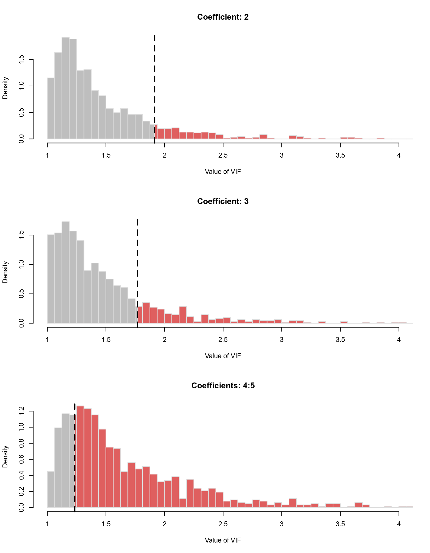
The vertical dashed lines indicate the observed (G)VIF values, which we can see are relatively large for the second and third model coefficients, corresponding to the year and ablat variables.
As a simpler approach, an examination of the correlations among the predictor variables does indicate some rather high correlations (between year and ablat, but also between the two dummy variables to represent the alloc factor, but the latter is to be expected given how such dummy variables are coded).
round(cor(model.matrix(res)[,-1]), digits=2)
                         year ablat factor(alloc)random factor(alloc)systematic
year                     1.00 -0.66               -0.13                    0.24
ablat                   -0.66  1.00                0.20                   -0.09
factor(alloc)random     -0.13  0.20                1.00                   -0.72
factor(alloc)systematic  0.24 -0.09               -0.72                    1.00
In any case, multicollinearity is certainly an explanation for the phenomenon illustrated above (where the omnibus test is significant, but none of the individual predictors are).
References
Bangert-Drowns, R. L., Hurley, M. M., & Wilkinson, B. (2004). The effects of school-based writing-to-learn interventions on academic achievement: A meta-analysis. Review of Educational Research, 74(1), 29-–58.
Colditz, G. A., Brewer, T. F., Berkey, C. S., Wilson, M. E., Burdick, E., Fineberg, H. V., et al. (1994). Efficacy of BCG vaccine in the prevention of tuberculosis: Meta-analysis of the published literature. Journal of the American Medical Association, 271(9), 698–702.