The metafor Package

Longitudinal or growth curve data (where individuals are repeatedly measured over time) are often analyzed using (linear) mixed-effects models. It can be instructional to examine how the results from such models can be approximated by a (simpler) two-stage analysis (e.g., section 4.2.3 in Diggle et al., 2002; section 3.2 in Verbeke & Molenberghs, 2000; Stukel & Demidenko, 1997).

As an illustration, we can use the Orthodont data from the nlme package:

library(nlme)
head(Orthodont)

Grouped Data: distance ~ age | Subject
  distance age Subject  Sex
1     26.0   8     M01 Male
2     25.0  10     M01 Male
3     29.0  12     M01 Male
4     31.0  14     M01 Male
5     21.5   8     M02 Male
6     22.5  10     M02 Male

The distance (in mm) from the pituitary to the pterygomaxillary fissure was measured four times for each of the 27 subjects (16 males and 11 females).

For easier interpretation of the results to be shown below, we can first "center" the age variable with:

Orthodont$age <- Orthodont$age - 8

That way, model intercepts will reflect the (average) distance at age 8.

Now, let's fit a standard linear mixed-effects model to these data, allowing the intercepts and slopes to (randomly) vary across subjects (also sometimes called a random intercepts and slopes model):

res1 <- lme(distance ~ age, random = ~ age | Subject, data=Orthodont)
summary(res1)

The results are:

Linear mixed-effects model fit by REML
 Data: Orthodont
       AIC      BIC    logLik
  454.6367 470.6173 -221.3183
 
Random effects:
 Formula: ~age | Subject
 Structure: General positive-definite, Log-Cholesky parametrization
            StdDev   Corr
(Intercept) 1.886629 (Intr)
age         0.226428 0.209
Residual    1.310039
 
Fixed effects: distance ~ age
                Value Std.Error DF  t-value p-value
(Intercept) 22.042593 0.4199079 80 52.49387       0
age          0.660185 0.0712533 80  9.26533       0
 Correlation:
    (Intr)
age -0.208
 
Standardized Within-Group Residuals:
         Min           Q1          Med           Q3          Max
-3.223105127 -0.493761346  0.007316611  0.472151021  3.916033671
 
Number of Observations: 108
Number of Groups: 27

Therefore, the estimated average distance at age 8 is $b_0 = 22.04$ millimeters ($SE = .420$). For each year, the distance is estimated to increase on average by $b_1 = 0.66$ millimeters ($SE = .071$). However, there is variability in the intercepts and slopes, as reflected by their estimated standard deviations ($SD(b_{0i}) = 1.887$ and $SD(b_{1i}) = 0.226$, respectively). Also, intercepts and slopes appear to be somewhat correlated ($\hat{\rho} = .21$). Finally, residual variability remains (reflecting deviations of the measurements from the subject-specific regression lines), as given by the residual standard deviation of $\hat{\sigma} = 1.310$.

Now let's use a two-stage approach to analyze these data. First, the linear regression model is fitted to the data for each person separately (i.e., based on the four observations per individual):

res.list <- lmList(distance ~ age, data=Orthodont)

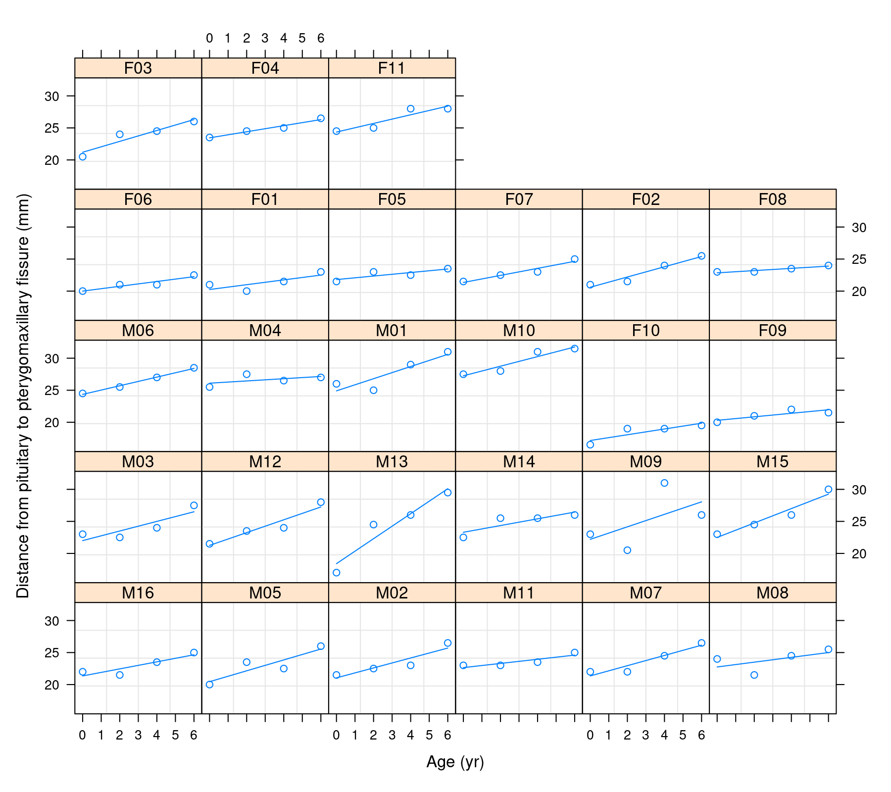
We can examine the individual profiles and fitted regression lines for each individual with:

plot(augPred(res.list), grid=TRUE)

From that object, we can extract the estimated model coefficients (intercepts and slopes) and the corresponding variance-covariance matrices with:

b <- lapply(res.list, coef)
V <- lapply(res.list, vcov)

A dummy variable indicating the estimate type (alternating intercept and slope) and a subject id variable are also needed, which can be created with:

estm <- rep(c("intercept","slope"), length(b))
subj <- rep(names(b), each=2)

Next, we create one long vector with the model coefficients and the corresponding block-diagonal variance-covariance matrix with (the metafor package needs to be loaded for the bldiag() function):

library(metafor)
b <- unlist(b)
V <- bldiag(V)

Finally, we conduct a multivariate meta-analysis with the model coefficients (since we have two correlated coefficients per subject). The V matrix contains the variances and covariances of the sampling errors. We also allow for heterogeneity in the true outcomes (i.e., coefficients) and allow them to be correlated (by using an unstructured variance-covariance matrix for the true outcomes). The model can be fitted with:

res2 <- rma.mv(b ~ estm - 1, V, random = ~ estm | subj, struct="UN")
res2

The results are:

Multivariate Meta-Analysis Model (k = 54; method: REML)
 
Variance Components:
 
outer factor: subj (nlvls = 27)
inner factor: estm (nlvls = 2)
 
            estim    sqrt  k.lvl  fixed      level
tau^2.1    3.9465  1.9866     27     no  intercept
tau^2.2    0.0478  0.2187     27     no      slope
 
           rho.intr  rho.slop    intr  slop
intercept         1    0.1959       -    no
slope        0.1959         1      27     -
 
Test for Residual Heterogeneity:
QE(df = 52) = 1611.6315, p-val < .0001
 
Test of Moderators (coefficient(s) 1,2):
QM(df = 2) = 3080.0214, p-val < .0001
 
Model Results:
 
               estimate      se     zval    pval    ci.lb    ci.ub
estmintercept   22.2769  0.4104  54.2826  <.0001  21.4725  23.0812  ***
estmslope        0.5762  0.0555  10.3868  <.0001   0.4675   0.6850  ***
 
---
Signif. codes:  0 ‘***’ 0.001 ‘**’ 0.01 ‘*’ 0.05 ‘.’ 0.1 ‘ ’ 1

The results are similar to the ones obtained earlier using the one-stage approach, with an estimated average intercept of $b_0 = 22.28$ ($SE = .410$), an estimated average slope of $b_1 = .58$ ($SE = .056$), estimated standard deviations of the underlying true intercepts and slopes equal to $SD(b_{0i}) = 1.987$ and $SD(b_{1i}) = 0.219$, respectively, and a correlation between the underlying true intercepts and slopes equal to $\hat{\rho} = .20$ (no residual standard deviation is given, since that source of variability is already incorporated into the V matrix).

This example illustrates how a two-stage procedure (i.e., fit the "level 1 model" per person, then aggregate the coefficients using essentially a meta-analytic model with corresponding random effects) is quite similar to what a mixed-effects model does. There are of course some underlying differences and the mixed-effects model approach should be more efficient. However, as described by Stukel and Demidenko (1997), there are circumstances where the two-stage approach is more robust to certain forms of model misspecification (when interest is focused on a subset of the model coefficients or some functions thereof).

Diggle, P. J., Heagerty, P., Liang, K.-Y., & Zeger, S. L. (2002). Analysis of longitudinal data (2nd ed.). Oxford: Oxford University Press.

Stukel, T. A., & Demidenko, E. (1997). Two-stage method of estimation for general linear growth curve models. Biometrics, 53(2), 720–728.

Verbeke, G., & Molenberghs, G. (2000). Linear mixed models for longitudinal data. New York: Springer.