Table of Contents
Forest Plot in RevMan Style
Description
Different software for meta-analysis draws forest plots in different styles and includes various pieces of information in the figure. For example, the figure below was created using RevMan, the software provided by the Cochrane Collaboration for conducting and authoring Cochrane reviews.
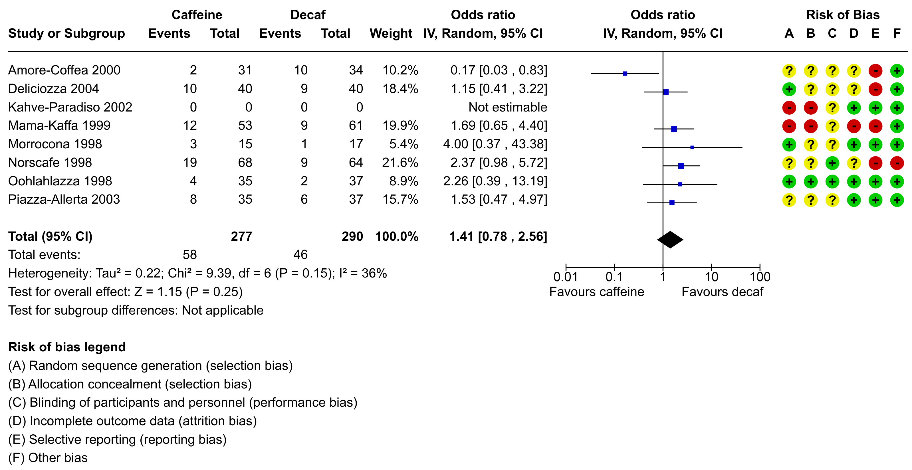
One of the strengths of R is its flexibility when creating figures. The code below shows how the figure can be recreated using a combination of the forest() function from metafor and using functions such as text() and points() to add additional elements to the figure in the same style as done in the RevMan forest plot. Note that it takes a bit of work to recreate the figure, although some parts are really optional (the goal here was to recreate the figure as closely as possible, except for a few minor deviations in terms of the alignment of the elements). Also note that one really needs to save the figure to a file for it to look right. The figure below was saved with png(filename="forest_plot_revman.png", res=350, width=3196, height=1648).
Plot
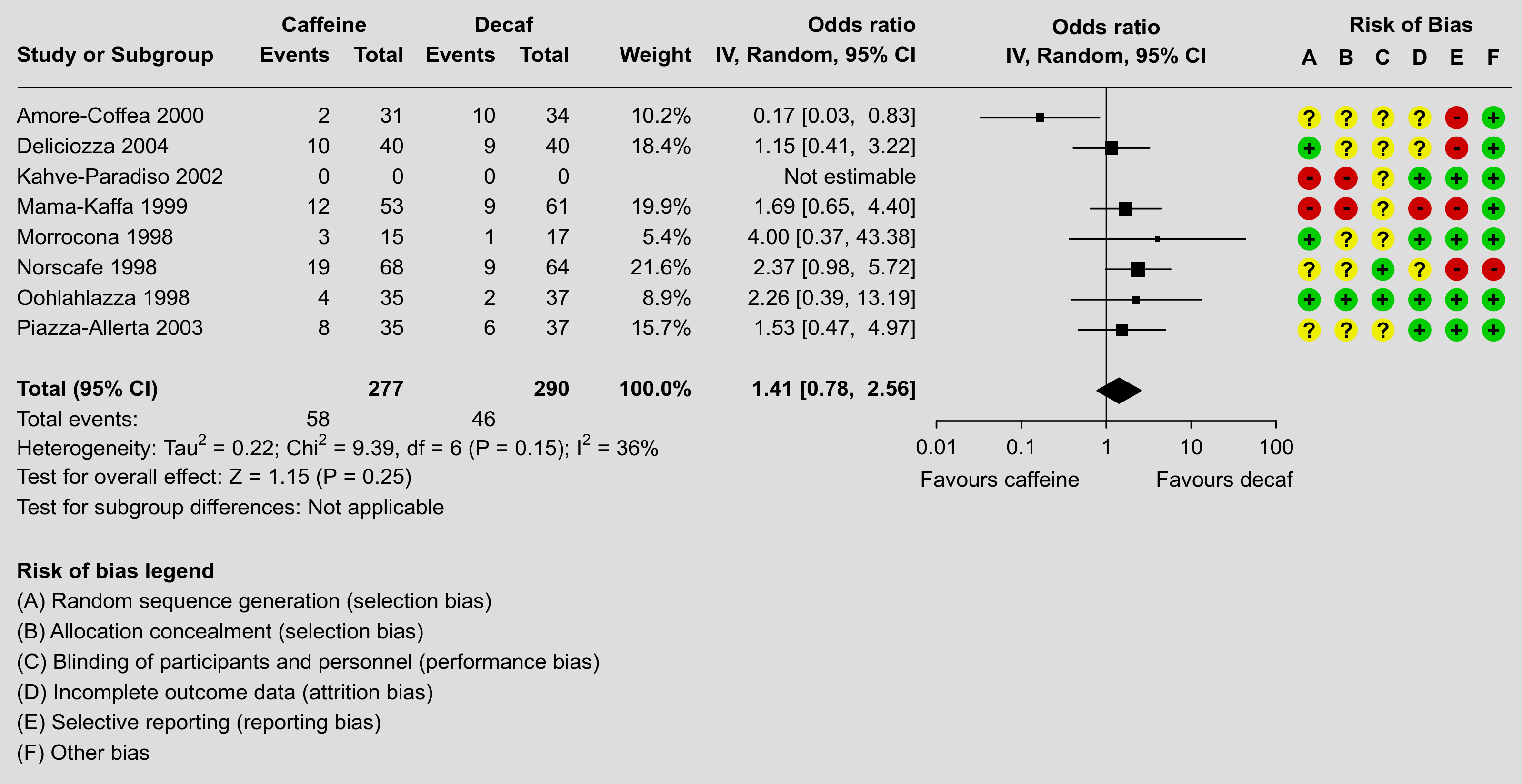
Code
### create the dataset
dat <- data.frame(author = c("Amore-Coffea", "Deliciozza", "Kahve-Paradiso", "Mama-Kaffa", "Morrocona", "Norscafe", "Oohlahlazza", "Piazza-Allerta"),
                  year   = c(2000, 2004, 2002, 1999, 1998, 1998, 1998, 2003),
                  ai     = c(2, 10, 0, 12, 3, 19, 4, 8),
                  n1i    = c(31, 40, 0, 53, 15, 68, 35, 35),
                  ci     = c(10, 9, 0, 9, 1, 9, 2, 6),
                  n2i    = c(34, 40, 0, 61, 17, 64, 37, 37),
                  rb.a   = c("?", "+", "-", "-", "+", "?", "+", "?"),
                  rb.b   = c("?", "?", "-", "-", "?", "?", "+", "?"),
                  rb.c   = c("?", "?", "?", "?", "?", "+", "+", "?"),
                  rb.d   = c("?", "?", "+", "-", "+", "?", "+", "+"),
                  rb.e   = c("-", "-", "+", "-", "+", "-", "+", "+"),
                  rb.f   = c("+", "+", "+", "+", "+", "-", "+", "+"))

### turn the risk of bias items into factors with levels +, -, and ?
dat[7:12] <- lapply(dat[7:12], factor, levels=c("+", "-", "?"))

### calculate log odds ratios and corresponding sampling variances (and use
### the 'slab' argument to store study labels as part of the data frame)
dat <- escalc(measure="OR", ai=ai, n1i=n1i, ci=ci, n2i=n2i, data=dat,
              slab=paste(author, year), drop00=TRUE)
dat

### note: using drop00=TRUE to leave the log odds ratio missing for the study
### with no events in either group (note the NAs for study 3)

### fit random-effects model (using the DL estimator as RevMan does)
res <- rma(yi, vi, data=dat, method="DL")
res

### estimated average odds ratio (and 95% CI/PI)
pred <- predict(res, transf=exp, digits=2)
pred

############################################################################

### need the rounded estimate and CI bounds further below
pred <- fmtx(c(pred$pred, pred$ci.lb, pred$ci.ub), digits=2)

### total number of studies
k <- nrow(dat)

### set na.action to "na.pass" (instead of the default, which is "na.omit"),
### so that even study 3 (with a missing log odds ratio) will be shown in the
### forest plot
options(na.action = "na.pass")

### get the weights and format them as will be used in the forest plot
weights <- paste0(fmtx(weights(res), digits=1), "%")
weights[weights == "NA%"] <- ""

### adjust the margins
par(mar=c(10.9,0,1.8,1.3), mgp=c(3,0.2,0), tcl=-0.2)

### forest plot with extra annotations
sav <- forest(res, atransf=exp, at=log(c(0.01, 0.10, 1, 10, 100)), xlim=c(-30,11),
       xlab="", efac=c(0,4), textpos=c(-30,-4.7), lty=c(1,1,0), refline=NA,
       ilab=cbind(ai, n1i, ci, n2i, weights),
       ilab.xpos=c(-20.6,-18.6,-16.1,-14.1,-10.8), ilab.pos=2,
       cex=0.78, header=c("Study or Subgroup","IV, Random, 95% CI"), mlab="",
       colout="#0000cc", colci="black")

### add horizontal line at the top
segments(sav$xlim[1]+0.5, k+1, sav$xlim[2], k+1, lwd=0.8)

### add vertical reference line at 0
segments(0, -2, 0, k+1, lwd=0.8)

### now we add a bunch of text; since some of the text falls outside of the
### plot region, we set xpd=NA so nothing gets clipped
par(xpd=NA)

### adjust cex as used in the forest plot and use a bold font
par(cex=sav$cex, font=2)

text(sav$ilab.xpos, k+2, pos=2, c("Events","Total","Events","Total","Weight"))
text(c(mean(sav$ilab.xpos[1:2]),mean(sav$ilab.xpos[3:4])), k+3, pos=2, c("Caffeine","Decaf"))
text(sav$textpos[2], k+3, "Odds ratio", pos=2)
text(0, k+3, "Odds ratio")
text(sav$xlim[2]-0.6, k+3, "Risk of Bias", pos=2)
text(0, k+2, "IV, Random, 95% CI")
text(c(sav$xlim[1],sav$ilab.xpos[c(2,4,5)]), -1, pos=c(4,2,2,2,2),
     c("Total (95% CI)", sum(dat$n1i), sum(dat$n2i), "100.0%"))
text(sav$xlim[1], -7, pos=4, "Risk of bias legend")

### first hide the non-bold summary estimate text and then add it back in bold font
rect(sav$textpos[2], -1.5, sav$ilab.xpos[5], -0.5, col="white", border=NA)
text(sav$textpos[2], -1, paste0(pred[1], " [", pred[2], ",  ", pred[3], "]"), pos=2)

### use a non-bold font for the rest of the text
par(cex=sav$cex, font=1)

### add 'Favours caffeine'/'Favours decaf' text below the x-axis
text(log(c(0.01, 100)), -4, c("Favours caffeine","Favours decaf"), pos=c(4,2), offset=-0.5)

### add 'Not estimable' for the study with missing log odds ratio
text(sav$textpos[2], k+1-which(is.na(dat$yi)), "Not estimable", pos=2)

### add text for total events
text(sav$xlim[1], -2, pos=4, "Total events:")
text(sav$ilab.xpos[c(1,3)], -2, c(sum(dat$ai),sum(dat$ci)), pos=2)

### add text with heterogeneity statistics
text(sav$xlim[1], -3, pos=4, bquote(paste("Heterogeneity: ",
   "Tau"^2, " = ", .(fmtx(res$tau2, digits=2)), "; ",
   "Chi"^2, " = ", .(fmtx(res$QE, digits=2)),
   ", df = ", .(res$k - res$p),
   " (", .(fmtp(res$QEp, digits=2, pname="P", add0=TRUE, sep=TRUE, equal=TRUE)), "); ",
   I^2, " = ", .(round(res$I2)), "%")))

### add text for test of overall effect
text(sav$xlim[1], -4, pos=4, bquote(paste("Test for overall effect: ",
   "Z = ", .(fmtx(res$zval, digits=2)),
   " (", .(fmtp(res$pval, digits=2, pname="P", add0=TRUE, sep=TRUE, equal=TRUE)), ")")))

### add text for test of subgroup differences
text(sav$xlim[1], -5, pos=4, bquote(paste("Test for subgroup differences: Not applicable")))

### add risk of bias points and symbols
cols <- c("#00cc00", "#cc0000", "#eeee00")
syms <- levels(dat$rb.a)
pos  <- seq(sav$xlim[2]-5.5,sav$xlim[2]-0.5,length=6)
for (i in 1:6) {
   points(rep(pos[i],k), k:1, pch=19, col=cols[dat[[6+i]]], cex=2.2)
   text(pos[i], k:1, syms[dat[[6+i]]], font=2)
}
text(pos, k+2, c("A","B","C","D","E","F"), font=2)

### add risk of bias legend
text(sav$xlim[1], -8:-13, pos=4, c(
   "(A) Random sequence generation (selection bias)",
   "(B) Allocation concealment (selection bias)",
   "(C) Blinding of participants and personnel (performance bias)",
   "(D) Incomplete outcome data (attrition bias)",
   "(E) Selective reporting (reporting bias)",
   "(F) Other bias"))