Table of Contents
Bootstrapping with Meta-Analytic Models
The use of bootstrapping in the meta-analytic context has been discussed by a number of authors (e.g., Adams, Gurevitch, & Rosenberg, 1997; van den Noortgate & Onghena, 2005; Switzer, Paese, & Drasgow, 1992; Turner et al., 2000). The example below shows how to conduct parametric and non-parametric bootstrapping using the metafor and boot packages in combination. The example is based on a meta-analysis by Collins et al. (1985) examining the effectiveness of diuretics in pregnancy for preventing pre-eclampsia.
Data Preparation
The data can be loaded with:
library(metafor)
dat <- dat.collins1985b[1:7]
dat
We only need the first 7 columns of the dataset (the remaining columns pertain to other outcomes). The contents of the dataset are:
  id                  author year pre.nti pre.nci pre.xti pre.xci
1  1       Weseley & Douglas 1962     131     136      14      14
2  2          Flowers et al. 1962     385     134      21      17
3  3                 Menzies 1964      57      48      14      24
4  4           Fallis et al. 1964      38      40       6      18
5  5         Cuadros & Tatum 1964    1011     760      12      35
6  6        Landesman et al. 1965    1370    1336     138     175
7  7            Kraus et al. 1966     506     524      15      20
8  8    Tervila & Vartiainen 1971     108     103       6       2
9  9 Campbell & MacGillivray 1975     153     102      65      40
Variables pre.nti and pre.nci indicate the number of women in the treatment and control/placebo groups, respectively, while pre.xti and pre.xci indicate the number of women in the respective groups with any form of pre-eclampsia during the pregnancy.
The corresponding log odds ratios (and corresponding sampling variances) can be computed and added to the dataset with:
dat <- escalc(measure="OR", ai=pre.xti, n1i=pre.nti, ci=pre.xci, n2i=pre.nci, data=dat)
dat
  id                  author year pre.nti pre.nci pre.xti pre.xci      yi     vi
1  1       Weseley & Douglas 1962     131     136      14      14  0.0418 0.1596
2  2          Flowers et al. 1962     385     134      21      17 -0.9237 0.1177
3  3                 Menzies 1964      57      48      14      24 -1.1221 0.1780
4  4           Fallis et al. 1964      38      40       6      18 -1.4733 0.2989
5  5         Cuadros & Tatum 1964    1011     760      12      35 -1.3910 0.1143
6  6        Landesman et al. 1965    1370    1336     138     175 -0.2969 0.0146
7  7            Kraus et al. 1966     506     524      15      20 -0.2615 0.1207
8  8    Tervila & Vartiainen 1971     108     103       6       2  1.0888 0.6864
9  9 Campbell & MacGillivray 1975     153     102      65      40  0.1353 0.0679
Random-Effects Model
For the analyses to be shown below, we will focus on the meta-analytic random-effects model, letting $y_i$ denote the observed outcome/effect for a particular study (variable yi in the dataset above) and $\theta_i$ the corresponding true outcome/effect. We assume that $$y_i = \theta_i + e_i,$$ where $e_i \sim N(0, v_i)$ denotes sampling error, whose variance is (approximately) known (variable vi in the dataset above). The true effects are in turn assumed to be given by $$\theta_i = \mu + u_i,$$ where $u_i \sim N(0, \tau^2)$, so that $\mu$ denotes the average true outcome/effect and $\tau^2$ the variance in the true outcomes/effects. The model implies that $$y_i \sim N(\mu, \tau^2 + v_i).$$ The goal is to estimate $\mu$ and $\tau^2$ and to construct corresponding confidence intervals for these parameters.
The results from fitting a random-effects model (using REML estimation) to the data given above can be obtained with:
res <- rma(yi, vi, data=dat)
res
Random-Effects Model (k = 9; tau^2 estimator: REML)

tau^2 (estimated amount of total heterogeneity): 0.3008 (SE = 0.2201)
tau (square root of estimated tau^2 value):      0.5484
I^2 (total heterogeneity / total variability):   75.92%
H^2 (total variability / sampling variability):  4.15

Test for Heterogeneity:
Q(df = 8) = 27.2649, p-val = 0.0006

Model Results:

estimate      se     zval    pval    ci.lb    ci.ub
 -0.5181  0.2236  -2.3167  0.0205  -0.9564  -0.0798  *

---
Signif. codes:  0 ‘***’ 0.001 ‘**’ 0.01 ‘*’ 0.05 ‘.’ 0.1 ‘ ’ 1
Therefore, the estimated average log odds ratio is equal to $\hat{\mu} = -.52$ with an approximate (Wald-type) 95% CI of $(-0.96, -0.08)$. The variance of the true log odds ratios is estimated to be $\hat{\tau}^2 = .30$. Confidence intervals for $\tau^2$ can be obtained in a variety of ways – see Viechtbauer (2007) for an illustration of a variety of different methods. One of them is the so-called Q-profile method, which provides exact CIs (under the assumptions of the model). Using this method, the CI bounds can be obtained with:
confint(res)
       estimate   ci.lb   ci.ub
tau^2    0.3008  0.0723  2.2027
tau      0.5484  0.2689  1.4842
I^2(%)  75.9238 43.1209 95.8494
H^2      4.1535  1.7581 24.0929
Note that CIs for the $I^2$ and $H^2$ statistics are also provided.
Parametric Bootstrapping
We will now use the boot package to obtain parametric and non-parametric bootstrap CIs for $\mu$ and $\tau^2$, so we start by loading the package with:
library(boot)
For parametric bootstrapping, we need to define two functions, one for calculating the statistic(s) of interest (and possibly the corresponding variance(s)) based on the bootstrap data, the second for actually generating the bootstrap data. In the present case, our interest is focused on the estimates of $\mu$ and $\tau^2$, so the first function could be written as:
boot.func <- function(data.boot) {

   res <- try(suppressWarnings(rma(yi, vi, data=data.boot)), silent=TRUE)

   if (inherits(res, "try-error")) {
      NA
   } else {
      c(coef(res), vcov(res), res$tau2, res$se.tau2^2)
   }

}
The purpose of the try() function is to catch cases where the algorithm used to obtain the REML estimate of $\tau^2$ does not converge. Otherwise, the function returns the estimate of $\mu$, the corresponding variance, the estimate of $\tau^2$, and its corresponding variance.
For a random-effects model, the data generation process is described by the last equation given above, where the two unknown parameters are replaced by their corresponding estimates (i.e., based on the fitted model). Therefore, the second function needed for the parametric bootstrapping is:
data.gen <- function(dat, mle) {
   data.frame(yi=rnorm(nrow(dat), mle$mu, sqrt(mle$tau2 + dat$vi)), vi=dat$vi)
}
Next, we can do the actual bootstrapping (based on 10,000 bootstrap samples) with (note that setting the seed allows for reproducibility of the results):
set.seed(8781328)
res.boot <- boot(dat, boot.func, R=10000, sim="parametric", ran.gen=data.gen, mle=list(mu=coef(res), tau2=res$tau2))
res.boot
PARAMETRIC BOOTSTRAP

Call:
boot(data = dat, statistic = boot.func, R = 10000, sim = "parametric",
    ran.gen = data.gen, mle = list(mu = coef(res), tau2 = res$tau2))

Bootstrap Statistics :
       original       bias    std. error
t1* -0.51810321  0.004338864  0.22661531
t2*  0.05001318 -0.000505738  0.02678718
t3*  0.30079577  0.003229987  0.22292854
t4*  0.04845165  0.013680859  0.07136553
Finally, a variety of different CIs for $\mu$ can be obtained with:
boot.ci(res.boot, type=c("norm", "basic", "stud", "perc"), index=1:2)
BOOTSTRAP CONFIDENCE INTERVAL CALCULATIONS
Based on 9964 bootstrap replicates

CALL :
boot.ci(boot.out = res.boot, type = c("norm", "basic", "stud",
    "perc"), index = 1:2)

Intervals :
Level      Normal              Basic
95%   (-0.9666, -0.0783 )   (-0.9604, -0.0720 )

Level    Studentized          Percentile
95%   (-1.0661,  0.0241 )   (-0.9642, -0.0758 )
Calculations and Intervals on Original Scale
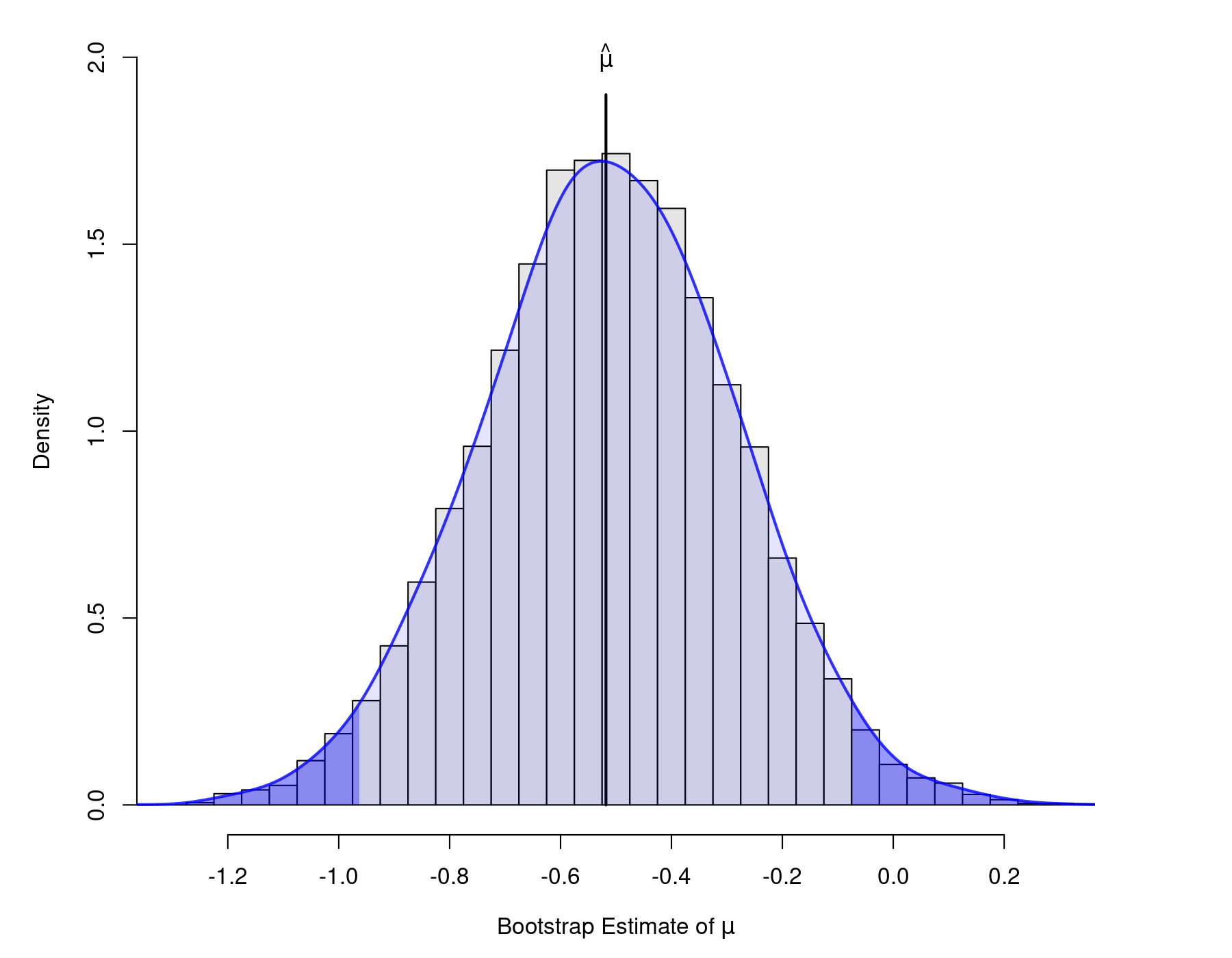
All of the intervals except the one based on the studentized method are similar to the Wald-type CI obtained earlier. The plot below shows the bootstrap distribution of $\hat{\mu}$ (with a kernel density estimate of the distribution superimposed and the tails shaded based on the percentile CI).

Since the studentized method is based on the use of the t-distribution, it is not surprising that more comparable results to the studentized CI can be obtained by using the Knapp and Hartung method when fitting the random-effects model (which also leads to the use of the t-distribution when constructing CIs for the fixed effects of the model). In particular, this can be done with:
rma(yi, vi, data=dat, test="knha")
Model Results:

estimate      se     tval    pval    ci.lb   ci.ub
 -0.5181  0.2408  -2.1512  0.0637  -1.0735  0.0373
The CI obtained in this manner is more similar to the one obtained using the studentized method.
Next, parametric bootstrap CIs for $\tau^2$ can be obtained with:
boot.ci(res.boot, type=c("norm", "basic", "stud", "perc"), index=3:4)
BOOTSTRAP CONFIDENCE INTERVAL CALCULATIONS
Based on 9964 bootstrap replicates

CALL :
boot.ci(boot.out = res.boot, type = c("norm", "basic", "stud",
    "perc"), index = 3:4)

Intervals :
Level      Normal              Basic
95%   (-0.1394,  0.7345 )   (-0.2358,  0.6016 )

Level    Studentized          Percentile
95%   ( 0.0644,  2.2430 )   ( 0.0000,  0.8374 )
Calculations and Intervals on Original Scale
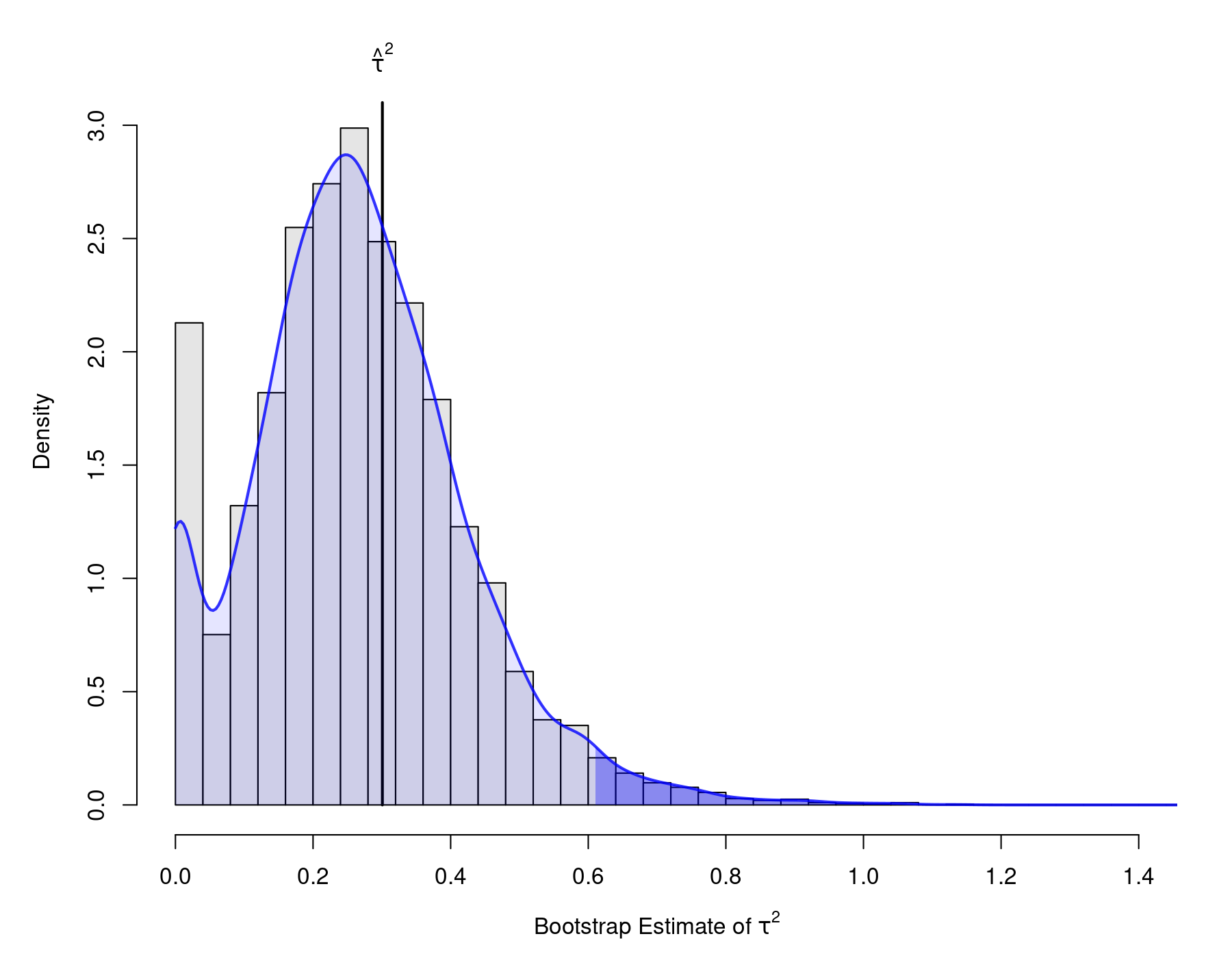
The various CIs are quite different from each other. Interestingly, the studentized method yields bounds that are quite similar to the ones obtained with the Q-profile method. Below is a plot of the bootstrap distribution of $\hat{\tau}^2$ (again, with the kernel density estimate and the tail regions shaded based on the percentile CI).

Non-Parametric Bootstrapping
For the non-parametric bootstrap method, we only need to define one function with two arguments, one for the original data and one for a vector of indices which define the bootstrap sample. The function again returns the statistics of interest (and the corresponding variances):
boot.func <- function(dat, indices) {

   sel <- dat[indices,]
   res <- try(suppressWarnings(rma(yi, vi, data=sel)), silent=TRUE)

   if (inherits(res, "try-error")) {
      NA
   } else {
      c(coef(res), vcov(res), res$tau2, res$se.tau2^2)
   }

}
Again, the try() function is used to catch the occasional case of non-convergence.
The actual bootstrapping can then be carried out with:
set.seed(8781328)
res.boot <- boot(dat, boot.func, R=10000)
res.boot
ORDINARY NONPARAMETRIC BOOTSTRAP

Call:
boot(data = dat, statistic = boot.func, R = 10000)

Bootstrap Statistics :
       original       bias    std. error
t1* -0.51810321  0.010904640  0.21186361
t2*  0.05001318 -0.004274829  0.02227421
t3*  0.30079577 -0.036116734  0.15587508
t4*  0.04845165  0.001846657  0.04922070
The various non-parametric bootstrap CIs for $\mu$ can now be obtained with:
boot.ci(res.boot, index=1:2)
BOOTSTRAP CONFIDENCE INTERVAL CALCULATIONS
Based on 9975 bootstrap replicates

CALL :
boot.ci(boot.out = res.boot, index = 1:2)

Intervals :
Level      Normal              Basic             Studentized
95%   (-0.9443, -0.1138 )   (-0.9128, -0.0968 )   (-1.3175, -0.0347 )

Level     Percentile            BCa
95%   (-0.9394, -0.1234 )   (-0.9792, -0.1532 )
Calculations and Intervals on Original Scale
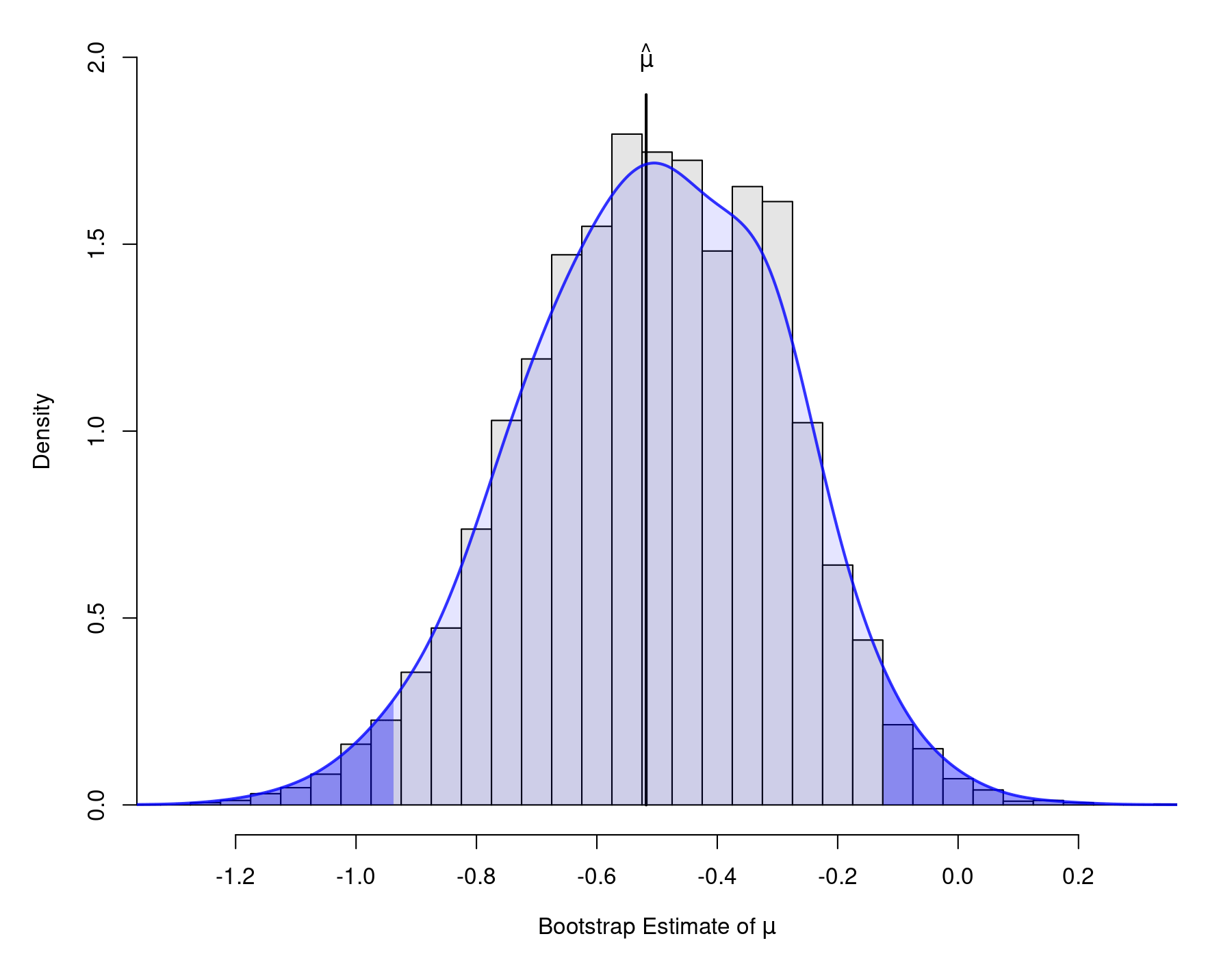
Now, the so-called bias-corrected and accelerated (BCa) CI is also included. The bootstrap distribution is shown below.

Finally, the various CIs for $\tau^2$ can be obtained with:
boot.ci(res.boot, index=3:4)
BOOTSTRAP CONFIDENCE INTERVAL CALCULATIONS
Based on 9980 bootstrap replicates

CALL :
boot.ci(boot.out = res.boot, index = 3:4)

Intervals :
Level      Normal              Basic             Studentized
95%   ( 0.0314,  0.6424 )   (-0.0104,  0.6016 )   ( 0.1381,  4.9414 )

Level     Percentile            BCa
95%   ( 0.0000,  0.6119 )   ( 0.0626,  0.8257 )
Calculations and Intervals on Original Scale
Again, the bootstrap distribution is shown below.

Discussion
The code above is shown for illustrative purposes only. Whether bootstrap CIs for $\mu$ are preferable to the standard Wald-type or Knapp-and-Hartung-adjusted CIs is unclear. Also, the results based on Viechtbauer (2007) suggest that the coverage probabilities of parametric and non-parametric bootstrap CIs for $\tau^2$ are less than adequate (however, only percentile and BCa intervals were closely examined in that paper, leaving the accuracy of the other bootstrap CIs unknown). Finally, other bootstrap strategies (e.g., the error bootstrap) are described by van den Noortgate and Onghena (2005).
References
Adams, D. C., Gurevitch, J., & Rosenberg, M. S. (1997). Resampling tests for meta-analysis of ecological data. Ecology, 78(5), 1277–1283.
Collins, R., Yusuf, S., & Peto, R. (1985). Overview of randomised trials of diuretics in pregnancy. British Medical Journal, 290(6461), 17–23.
van den Noortgate, W., & Onghena, P. (2005). Parametric and nonparametric bootstrap methods for meta-analysis. Behavior Research Methods, 37(1), 11–22.
Switzer III, F. S., Paese, P. W., & Drasgow, F. (1992). Bootstrap estimates of standard errors in validity generalization. Journal of Applied Psychology, 77(2), 123–129.
Turner, R. M., Omar, R. Z., Yang, M., Goldstein, H., & Thompson, S. G. (2000). A multilevel model framework for meta-analysis of clinical trials with binary outcomes. Statistics in Medicine, 19(24), 3417–3432.
Viechtbauer, W. (2007). Confidence intervals for the amount of heterogeneity in meta-analysis. Statistics in Medicine, 26(1), 37–52.