Table of Contents
Speeding Up Model Fitting
Fitting models to large datasets and/or models involving a large number of random effects (for the rma.mv() function) can be time consuming. Admittedly, some routines in the metafor package are not optimized for speed and efficient memory usage by default. However, there are various ways for speeding up the model fitting, which are discussed below.
Large Datasets
Most meta-analytic datasets are relatively small, with less than a few dozen studies (and often even much smaller than that). However, occasionally, one may deal with a much larger dataset, at which point the rma() (i.e., rma.uni()) function may start to behave sluggishly. To illustrate this, let's simulate a large dataset with $k = 4000$ studies based on a random-effects model (with $\mu = 0.50$ and $\tau^2 = 0.25$).
set.seed(132451)
k <- 4000
vi <- runif(k, 0.01, 1)
yi <- rnorm(k, 0.5, sqrt(vi + 0.25))
We then measure how long it takes to fit a random-effects model to these data.
library(metafor)
system.time(res <- rma(yi, vi))
   user  system elapsed
 565.14    1.87  567.03
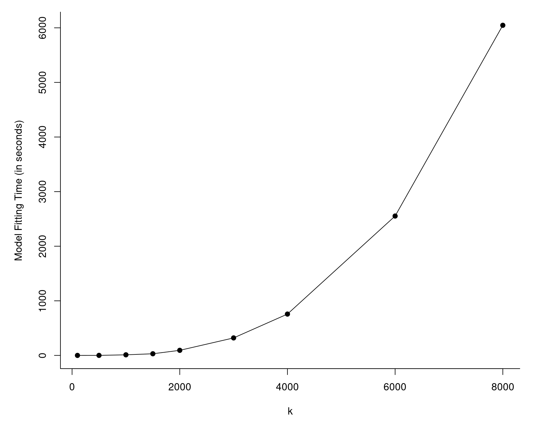
The values are given in seconds and the one we are interested in is the last one (the elapsed time). So, it took almost 10 minutes to fit this model, although this was on a pretty outdated workstation with an Intel Xeon E5430 CPU running at 2.67 Ghz. A more modern/faster CPU will crunch through this much quicker, but even larger values of $k$ will eventually lead to the same problem. In fact, the model fitting time will tend to increase at a roughly quadratic rate as a function of $k$, as can be seen in the figure below.

The reason for this is that rma() carries out some computations that involve $k \times k$ matrices. As these matrices grow in size, the time it takes to carry out the matrix algebra increases at a roughly quadratic rate. Note that this generally won't be an issue unless the number of studies is in the thousands, but at that point, model fitting can become really slow.
There are two ways of speeding up the model fitting in such a scenario. The first involves switching to the rma.mv() function, which we can also use for fitting the random-effects model (see also this comparison of the rma.uni() and rma.mv() functions for more details). Here, we can make use of the fact that the marginal variance-covariance matrix of the observed outcomes is actually very sparse (to be precise, it is diagonal). By setting the argument sparse=TRUE, sparse matrix objects are used to the extent possible, which can speed up model fitting substantially for certain models. The syntax for fitting the random-effects model would be:
id <- 1:k
system.time(res <- rma.mv(yi, vi, random = ~ 1 | id, sparse=TRUE))
   user  system elapsed
  40.09    1.05   41.14
So, instead of almost ten minutes, it now only took about 40 seconds, which is quite an improvement.
An alternative approach for speeding up the model fitting is to make use of optimized routines for the matrix algebra. The BLAS (Basic Linear Algebra Subprograms) library supplied with "vanilla R" is quite good, but enhanced linear algebra routines can be quite a bit faster. It is beyond the scope of this note to discuss how we can get R to make use of such enhanced routines, but the interested reader should take a look at the relevant section in the R Installation and Administration manual.
However, one of the easiest ways for getting the benefits of enhanced math routines is to install Microsoft R Open (MRO), which is a 100% compatible distribution of R (with a few added components), but most importantly, it provides the option to automatically install Intel's Math Kernel Library (MKL) alongside MRO. As the name implies, MKL will be most beneficial on Intel CPUs, so those with AMD processors may not see as much of a performance boost (or none at all? haven't tested this). At any rate, here are the results when fitting the model above with MRO+MKL using the rma() function.
system.time(res <- rma(yi, vi))
   user  system elapsed
  42.83    1.93   44.77
So, about 45 seconds, as opposed to almost 10 minutes with vanilla R. Interestingly, MRO+MKL is about as quick for this example as using vanilla R with rma.mv(..., sparse=TRUE). However, we can get even better performance with MKL if we allow for multicore processing (one of the benefits of MKL is that it can run multithreaded and hence make use of multiple cores). The workstation I am using for these analyses actually has two quad-core CPUs, so there are 8 cores available we can make use of. Using the setMKLthreads() command, we can set the number of cores that MKL is allowed to make use of. Let's see what happens if we give it all 8 cores.
setMKLthreads(8)
system.time(res <- rma(yi, vi))
   user  system elapsed
  68.72   10.77   11.63
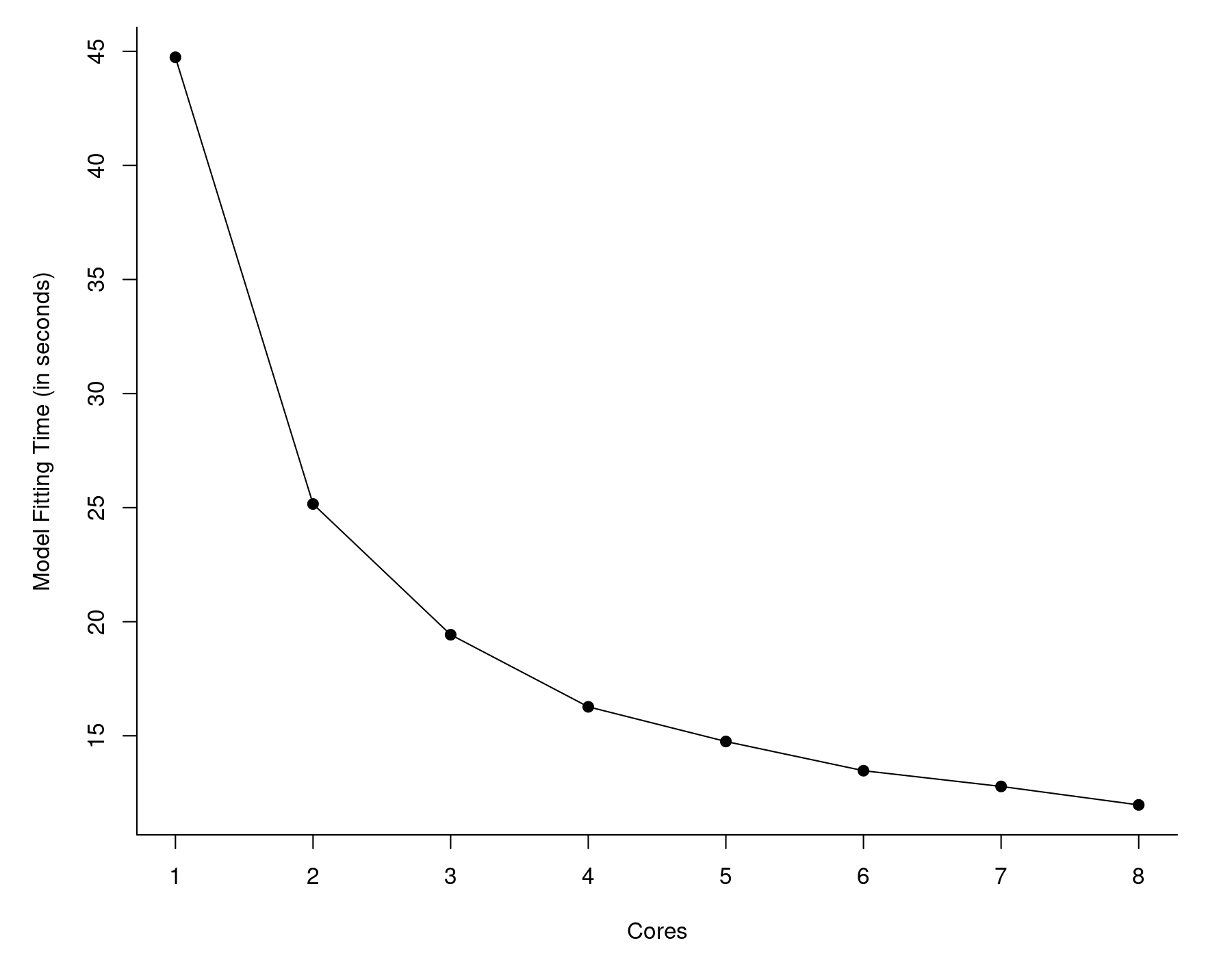
So now we are down to less than 12 seconds! That's almost 50 times faster than what we started out with (567 seconds). I also examined the model fitting time as a function of the number of cores we make available to MKL. The results are shown in the graph below.

With more cores, things do speed up, but the gains diminish as we add more cores. Also, with just a single core, MKL took about 45 seconds as opposed to vanilla R, which took almost 10 minutes. So the largest gains come from switching to MKL in the first place, not the use of multiple cores.
One can even try combining the use of MRO+MKL with rma.mv(..., sparse=TRUE). In this particular example, this didn't yield any additional performance benefits (and actually slowed things a little bit). I suspect that the performance benefits of MKL in this example are actually related to using numerical routines that can take advantage of the sparseness of the matrices automatically. Hence, there is no benefit in trying to exploit this characteristic of the data twice. However, with even larger values of $k$, use of rma.mv(..., sparse=TRUE) together with MKL can yield some additional benefits due to more efficient storage of the underlying matrices.
Complex Models
Fitting complex models with the rma.mv() function can also be time consuming. The most crucial aspect here is the number (and types) of random effects that are added to the model (the number of fixed effects is pretty much irrelevant for the underlying optimization routines). For illustration purposes, I simulated a large dataset based on a rather complex random effects structure. This dataset can be loaded directly into R with:
dat <- read.table("http://www.metafor-project.org/lib/exe/fetch.php/tips:data_complex_model.dat", header=TRUE, sep="\t")
For reasons to be explained shortly, we will also load two correlation matrices:
R.plant  <- read.table("http://www.metafor-project.org/lib/exe/fetch.php/tips:data_complex_model_R_plant.dat", header=TRUE, sep="\t")
R.fungus <- read.table("http://www.metafor-project.org/lib/exe/fetch.php/tips:data_complex_model_R_fungus.dat", header=TRUE, sep="\t")
First, let's look at the first 10 rows of the dataset.
head(dat, 10)
   study experiment plant fungus plant.phyl fungus.phyl     yi     vi
1      1          1   P07    F09        P07         F09  0.737 0.4985
2      1          2   P34    F22        P34         F22  1.947 0.5874
3      1          3   P14    F06        P14         F06 -0.573 0.4418
4      2          1   P27    F02        P27         F02 -0.266 0.1107
5      2          2   P27    F06        P27         F06 -0.317 0.0847
6      3          1   P19    F25        P19         F25 -0.051 0.2088
7      3          2   P14    F12        P14         F12  0.685 0.2195
8      3          3   P14    F06        P14         F06  1.374 0.0640
9      4          1   P25    F24        P25         F24  0.979 0.2103
10     4          2   P14    F24        P14         F24  1.288 0.3204
So, we have experiments nested within studies that were conducted with various combinations of plant species and fungi. We can familiarize ourselves a bit more with this dataset using the following commands.
nrow(dat)                    # number of rows (i.e., observed outcomes)
length(unique(dat$study))    # number of studies
table(table(dat$study))      # table of the number of experiments within studies
length(unique(dat$plant))    # number of plants
table(dat$plant)             # table of the number of outcomes per plant
length(unique(dat$fungus))   # number of fungi
table(dat$fungus)            # table of the number of outcomes per fungus
table(dat$plant, dat$fungus) # table of plant-fungus frequencies
The output (not shown) indicates that there are 2000 observed outcomes, 868 studies, and most studies included between 1 and 4 experiments. Furthermore, 35 different plant species were studied and 25 different fungi, each with different frequencies.
We will fit a three-level meta-analytic model to these data (with experiments nested within studies) with crossed random effects for the plant and fungus factors. In addition, the R.plant and R.fungus correlation matrices loaded earlier reflect phylogenetic correlations for the various plant species and fungi studied. Hence, we will include phylogenetic random effects in the model based on these correlation matrices. For more details on models of this type, see Konstantopoulos (2011) and Nakagawa and Santos (2012). The code for fitting such a model is shown below.
system.time(
res <- rma.mv(yi, vi, random = list(~ 1 | study/experiment,
                                    ~ 1 | plant,
                                    ~ 1 | fungus,
                                    ~ 1 | plant.phyl,
                                    ~ 1 | fungus.phyl),
              R = list(plant.phyl = R.plant, fungus.phyl = R.fungus),
              data = dat)
)
   user  system elapsed
5696.19   59.11 5755.53
So, using vanilla R, fitting this model on my workstation took about 95 minutes. Ouch!
Let's try speeding things up. Given the discussion above, one may be inclined to try the sparse=TRUE option. However, this yields:
    user   system  elapsed
23755.76   362.74 24120.41
So now it took almost 7 hours to fit the same model, so this attempt really backfired. The reason for this is that the underlying matrices that the optimization routine has to deal with are not sparse at all (due to the crossed and correlated random effects). Forcing the use of sparse matrices then creates additional (and unnecessary) overhead, leading to a substantial slowdown.
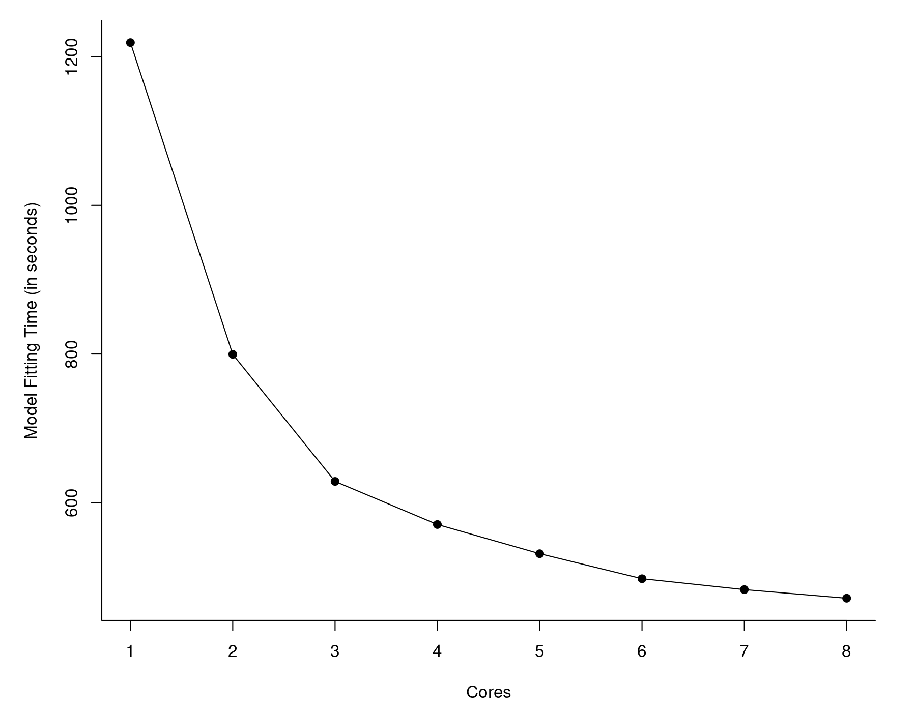
Instead, we can give MRO+MKL a try. As above, I examined the time it took to fit the model as a function of cores made available. These are the results:

So, even with just one core, MRO+MKL took about 20 minutes. Again, we see diminishing returns as we make more cores available to MKL, but with all 8 cores, the model fitting was down to less than 8 minutes. This is more than 12 times faster than vanilla R. Quite a difference.
Other Adjustments
A few other adjustments can be tried to speed up the model fitting. First of all, the rma.mv() function provides a lot of control over the optimization routine (see help(rma.mv) and especially the information about the control argument). For example, switching to a different optimizer may speed up the model fitting – but could also slow things down. So, whether this is useful is a matter of trial and error. Furthermore, the starting values for the optimization are not chosen in a terribly clever way at the moment and could be far off, in which case convergence may be slow. One can set the starting values manually via the control argument. This could be useful, for example, when fitting several different but similar models to the same dataset.
Final Comments
One thing I would like to clarify. The comparison between "vanilla R" and "MRO+MKL" is really a comparison between the reference BLAS library of R versus MKL (so vanilla R versus MRO is not the issue here). Note that there are other linear algebra libraries (especially ATLAS and OpenBLAS) that can also be used with R and that may provide similar speedups. If anybody has made comparisons between these different options in conjunction with metafor, I would be curious to hear about it.
References
Konstantopoulos, S. (2011). Fixed effects and variance components estimation in three-level meta-analysis. Research Synthesis Methods, 2(1), 61–76.
Nakagawa, S., & Santos, E. S. A. (2012). Methodological issues and advances in biological meta-analysis. Evolutionary Ecology, 26(5), 1253–1274.