The metafor Package

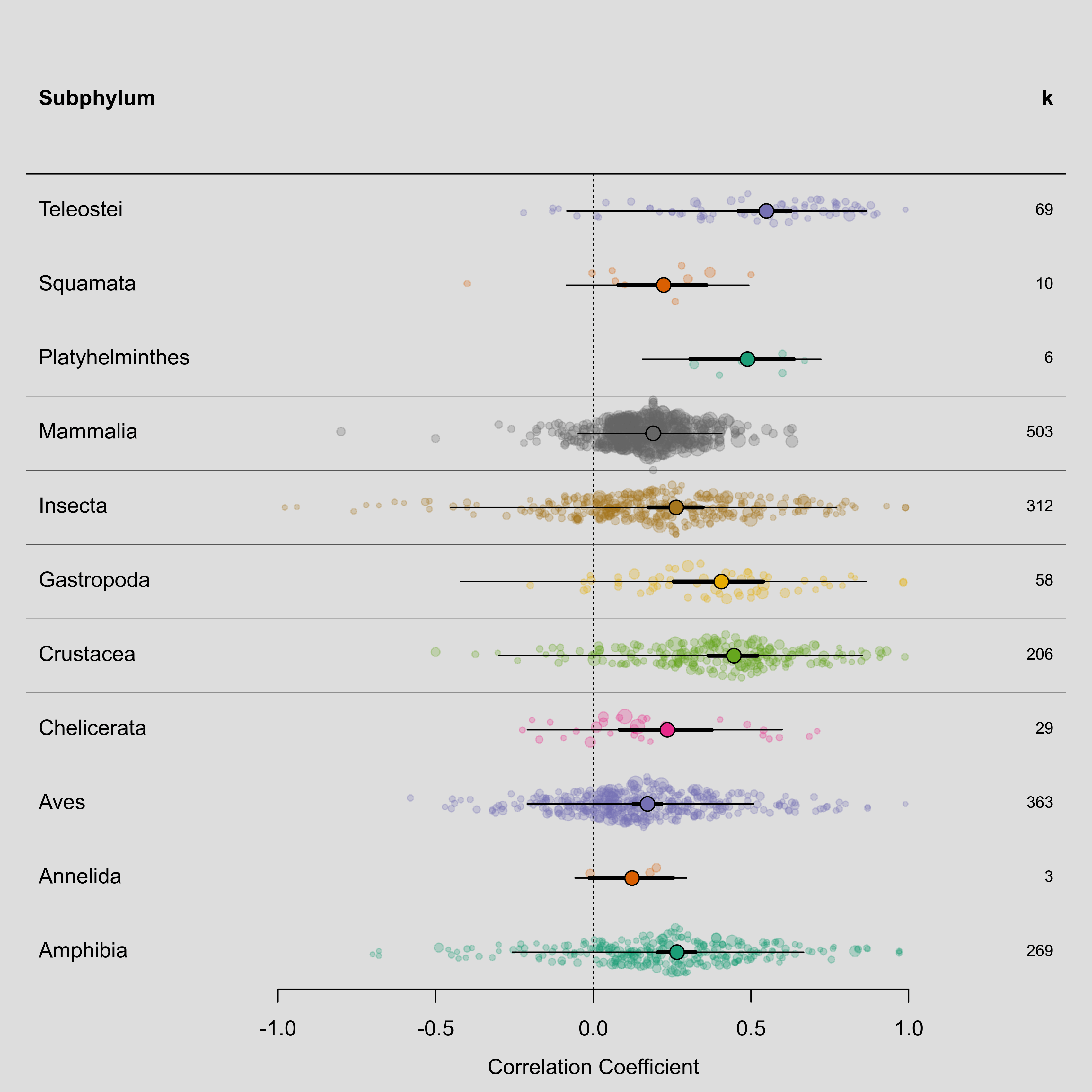
When dealing with large meta-analytic datasets, standard forest plots can become become excessively large (or the size of the elements in the plot become very small). To handle this problem, authors sometimes use forest-like plots that do not show the individual effect size estimates but instead the pooled estimate, often within the levels of a categorical moderator. However, as noted by Nakagawa et al. (2021), showing the individual estimates can still be informative. For this, they proposed ‘orchard plots’ that show the individual estimates (but without their corresponding 95% CIs) in a bee swarm style and then superimpose the pooled estimate and corresponding 95% CI/PI intervals on the points. The example below illustrates such a plot created with a combination of the forest() function and some base R plotting functions such as segments() and text(). Note that the orchaRd package can also be used to create such plots.

The example is based on the meta-analysis by Rios Moura et al. (2021) on assortative mating, examining the similarity of some measure of body size in mating couples. The meta-analysis included 457 studies, providing a total of 1828 correlation coefficients across 341 different species, which can be grouped into 11 different subphyla.

Note: At the moment, you will need to install the development version of the metafor package for the example to work, as I just recently added the colci argument to the various forest() functions in the package.

library(metafor)
 
### copy the data to 'dat'
dat <- dat.moura2021$dat
 
### calculate r-to-z transformed correlations and corresponding sampling variances
dat <- escalc(measure="ZCOR", ri=ri, ni=ni, data=dat)
 
### number of correlations per subphylum
table(dat$subphylum)
 
### number of levels
nlvls <- length(table(dat$subphylum))
 
### fit a multilevel model allowing variances to differ across the levels of subphylum
### (note: this takes a bit of time, so be patient)
res <- rma.mv(yi, vi, mods = ~ 0 + subphylum, 
              random = list(~ subphylum | study.id, ~ subphylum | effect.size.id), 
              struct="DIAG", sparse=TRUE, data=dat)
 
### generate the row values (this can be done in various ways; here the
### estimates closer to the pooled estimates are jittered more)
set.seed(1234)
dat$row <- as.numeric(factor(dat$subphylum))
d <- abs(resid(res))^(1/8)
d <- (d - min(d)) / (max(d) - min(d))
d <- (1 - d) * 0.5
dat$row.jitter <- dat$row + runif(nrow(dat), -d, d)
 
### generate the colors
cols <- rep(palette.colors(8, palette="Dark 2"), length.out=nlvls)
cols.adj <- adjustcolor(cols, alpha.f=0.6)
dat$colpt <- cols.adj[dat$row]
 
### optional: winsorize the sampling variances at the 5th percentile (to make
### differences in sampling variances across studies more visually apparent)
dat$viadj <- pmax(dat$vi, quantile(dat$vi, 0.05))
 
### draw the forest plot
sav <- with(dat, forest(yi, viadj, header="Subphylum", rows=row.jitter, slab=NA, 
                        annotate=FALSE, xlim=c(-1.8,1.5), ylim=c(0.5,nlvls+2.5), 
                        cex=1, pch=19, efac=0, col=colpt, colci=NA, 
                        transf=transf.ztor, digits=1))
text(sav$xlim[1], 1:nlvls, names(table(dat$subphylum)), pos=4)
abline(h=0:nlvls+0.5, col="gray20", lwd=0.2)
 
### add points/CIs/PIs for the different subphylum levels
pred <- predict(res, newmods=diag(res$p), tau2.levels=1:nlvls, 
                gamma2.levels=1:nlvls, transf=transf.ztor)
segments(pred$pi.lb, 1:nlvls, pred$pi.ub, 1:nlvls, lwd=1)
segments(pred$ci.lb, 1:nlvls, pred$ci.ub, 1:nlvls, lwd=3)
points(pred$pred, 1:nlvls, pch=21, bg=cols, cex=1.5)
 
### add the number of correlations for the different subphylum levels
text(sav$xlim[2], sav$ylim[2]-1, "k", pos=2, font=2)
text(sav$xlim[2], 1:nlvls, table(dat$subphylum), pos=2, cex=0.75)

Nakagawa, S., Lagisz, M., O’Dea, R. E., Rutkowska, J., Yang, Y., Noble, D. W. A., & Senior, A. M. (2021). The orchard plot: Cultivating a forest plot for use in ecology, evolution, and beyond. Research Synthesis Methods, 12(1), 4–12. https://doi.org/10.1002/jrsm.1424

Rios Moura, R., Oliveira Gonzaga, M., Silva Pinto, N., Vasconcellos-Neto, J., & Requena, G. S. (2021). Assortative mating in space and time: Patterns and biases. Ecology Letters, 24(5), 1089–1102. https://doi.org/10.1111/ele.13690