The metafor Package

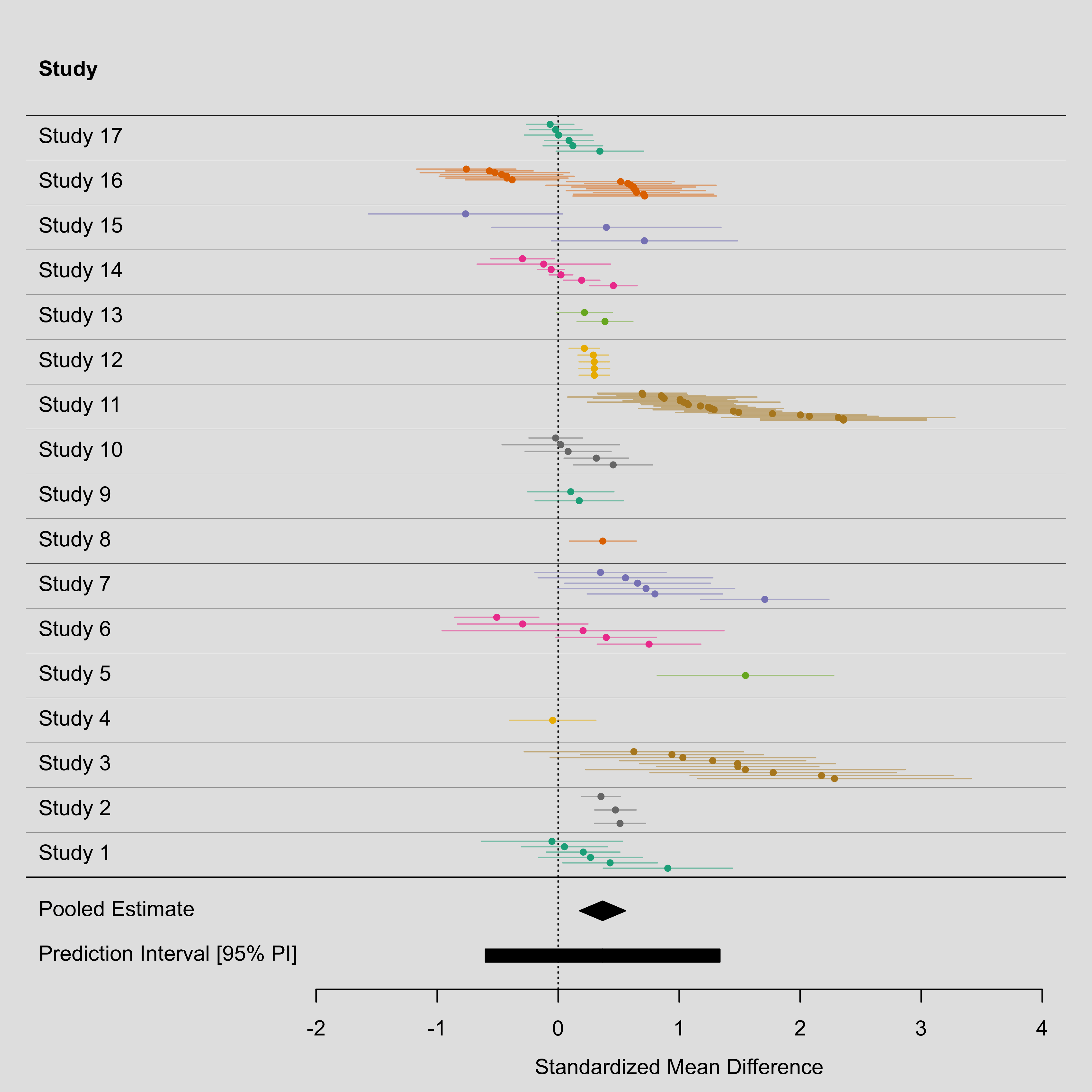
When dealing with large meta-analytic datasets where studies may contribute multiple effect size estimates to the same analysis, standard forest plots can become excessively large (or the size of the elements in the plot become very small). One possible solution to this problem is to group the estimates from the same study together, omitting the text annotations (i.e., the estimate and corresponding confidence interval bounds) for the individual estimates. A bit of color can be used to make the grouping of the estimates within studies more visually apparent.

The example below illustrates this possibility. It is based on the example dataset from Assink et al. (2015), which includes 100 estimates (standardized mean differences) on the difference in recidivism between delinquent juveniles with and without a mental health disorder.

Note: At the moment, you will need to install the development version of the metafor package for the example to work, as I just recently added the colci argument to the various forest() functions in the package.

library(metafor)
 
### copy the data to 'dat'
dat <- dat.assink2016
 
### assume that the effect sizes within studies are correlated with rho=0.6
V <- vcalc(vi, cluster=study, obs=esid, data=dat, rho=0.6)
 
### fit a multilevel model using this approximate V matrix
res <- rma.mv(yi, V, random = ~ 1 | study/esid, data=dat, digits=3)
res
 
### sort the estimates within each study
dat <- sort_by(dat, ~ study + yi, decreasing=TRUE)
 
### generate the row values
dat$row <- as.numeric(factor(dat$study))
dat$row.seq <- ave(dat$row, dat$row, FUN = function(x) {
   n <- length(x)
   x + if (n == 1) 0 else if (n == 2) c(-0.1, 0.1) else seq(-0.3, 0.3, length.out=n)
})
 
### generate the study labels
dat$slab <- paste("Study", dat$study)
dat$slab[duplicated(dat$slab)] <- ""
 
### generate tje colors
dat$colpt <- rep(rep(palette.colors(8, palette="Dark 2"), 
                 length.out=length(unique(dat$study))), times=rle(dat$study)$lengths)
dat$colci <- adjustcolor(dat$colpt, 0.5, 1, 1, 1)
 
### draw the forest plot
sav <- with(dat, forest(yi, vi, rows=row.seq, slab=NA, annotate=FALSE,
                        xlim=c(-4.4,4.2), ylim=c(-2.0,floor(max(dat$row))+2.5),
                        cex=1, pch=19, psize=0.8, efac=0, col=colpt, colci=colci))
text(sav$xlim[1], dat$row, dat$slab, pos=4)
abline(h=0:max(dat$row)+0.5, col="gray20", lwd=0.2)
 
### add the results from the model to the plot
addpoly(res, row=-0.25, efac=1, mlab="Pooled Estimate", predstyle="bar")
abline(h=0.5)